Review of Data Mining Algorithms

Algorithm Representation Usage Adv Disadv

Association Rule Prop if-then discover simple slow, rep,

correlations no oracle no predict

Decision Tree Disj of prediction robust prediction, overfit,

prop conj symbolic rules representation

Neural Network Nonlinear prediction numeric, overfit, slow,

numeric f(x) noisy data difficult to

interpret output

Naive Bayes Est prob prediction noisy data, not effective

provable answer in practice

Belief Network network & CPTs prediction, prior info, slow

variable influence prob dist learn structure

Nearest Neighbor Instances prediction no training, slow query,

no fixed bias redun attributes

no loss of info no bias

Clustering clusters discover correlations, no oracle, difficult to

discover var influence find similar features interpret output

find sim instances

Data Mining Applications

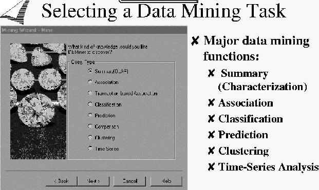
Image-Based Data Mining
- Job posting on Monday
- Analyze images for stroke, aging, trauma
Newswire Data mining
- Reuters Newswire (1987)
- 22,173 documents
- 135 keywords (countries, topics, people, organizations, stock exchanges)
- Background knowledge: 1995 CIA World Factbook (member of, land boundaries, natural resources, export commodities, export partners, industries, etc.)
- Iran, Nicaragua, USA $\rightarrow$ Reagan (6/1.0)
- Iran, USA $\rightarrow$ Reagan (18/0.692)
- gold, copper $\rightarrow$ Canada (5/0.625)
- gold, copper $\rightarrow$ USA (12/0.571)
- gold, copper $\rightarrow$ Switzerland (5/1.0)
- gold, copper $\rightarrow$ Belgium (5/1.0)
Churning (customer turnover) in telecommunications industry
- Cost of churn is approximately $400 per new subscriber
- Prediction (will this customer churn and when)
- Understanding (why do particular customers churn)
- Act (reduce churn rate by offering incentives)
- account length in days, international plan, voice mail, number of messages, length of day time calls, length of evening calls, length of night calls, length of international calls, customer service calls, churn status
- Clusters
  - International Users (no voice mail, high international usage)
  - Internet Users (no voice mail, high day, evening, night usage)
  - Busy Workers (no voice mail, low day and evening usage, high customer service calls)
  - Long term customers, long term voice mail customers, new customer

Data Preparation

KDD Process

The Problem

Data Preparation

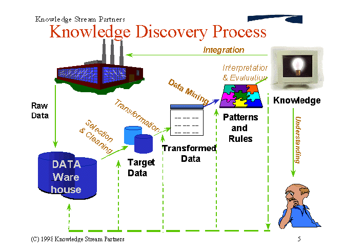
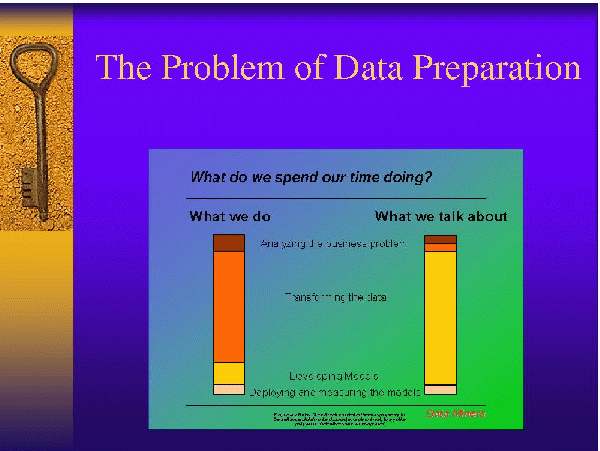
Convert data to desired format
Transform data
- Normalization
- Smoothing
- Data Reduction
  - Feature discretization
  - Sampling
  - Feature selection
- Feature composition
- Often requires human assistance to find best set of transformations
Dealing with Missing Data

Discretization of Continuous Features

A discretization algorithm converts continuous features into discrete features

$\psfig{figure=figures/disc1.ps}$

Motivation

1.: Some algorithms are limited to discrete inputs
2.: Many algorithm discretize as part of the learning algorithm, perhaps not in the best manner
3.: Continuous features drastically slow learning
4.: More easily view data

Types of discretization

Discretization can be classified on two dimensions

1.

Supervised vs. unsupervised
Supervised uses class information

2.

Global (mesh) vs. local

$\psfig{figure=figures/disc2.ps}$

One can apply some discretization methods either globally or locally

Single Feature Discretization

Here we consider only global discretization of single features.

1.: Limit scope of problem
Allowing discretization of multiple input features is as hard as entire induction problem
2.: Easy to interpret discretization

Equal Interval Width (Binning)

1.

Given k bins, divide the training-set range into k equal-size bins

$\psfig{figure=figures/disc3.ps}$

2.

Problems

(a): Unsupervised
(b): Where does k come from?
(c): Sensitive to outliers
$\psfig{figure=figures/disc4.ps}$

Equal Frequency

Split into intervals of equal size
Divide m instances into k bins, each containing m/k(possibly duplicated) values
This method is unsupervised
Not often used

A possible local unsupervised method: k-means clustering

OneR

Developed in 1993 by Holte
Used in OneR induction algorithm
Induces one-level decision trees (decision stumps)
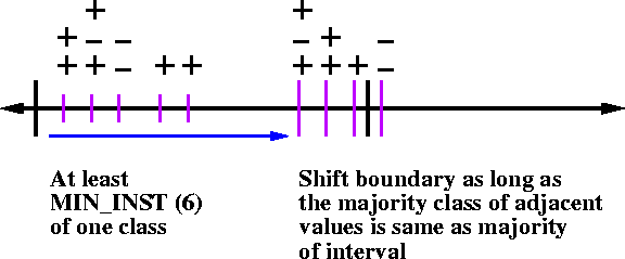
Divide range into pure bins
Each bin contains strong majority of a class
Each bin must include at least threshold number of instances
This method is supervised

$\psfig{figure=figures/disc5.ps}$

Minimal Entropy Partitioning

Developed in 1993 by Fayyad and Irani
Find best threshold split, such that mutual information between feature and label is maximal
Split data according to threshold
Given
- Set of instances S
- Feature A
- Partition boundary T
Class entropy of partition induced by T, E(A,T;S) is calculated as

$\begin{displaymath}E(A,T;S) \;=\; \frac{\mid S_1 \mid}{\mid S \mid} Ent(S_1) \;+\; \frac{\mid S_2 \mid}{\mid S \mid} Ent(S_2)\end{displaymath}$
Recursively discretize each partition
Stopping condition based on MDL Principle, stop when

$\begin{displaymath}Gain(A,T;S) \;<\; \frac{lg(N-1)}{N} \;+\; \frac{\Delta(A,T;S)}{N}\end{displaymath}$

where
- N is number of instances in set S
- Gain(A,T;S) = Ent(S) - E(E,A;S)
- $\Delta(A,T; S) \;=\; lg(3^k - 2) \;-\; (k*Ent(S) - k_1*Ent(S_1) - k_2*Ent(S_2))$
Run time is O(km lg m), space is O(m)

How many partitions? D2 (Catlett), MDL approach (Fayyad and Irani) offer answers.

This method is supervised.

Comparison 1

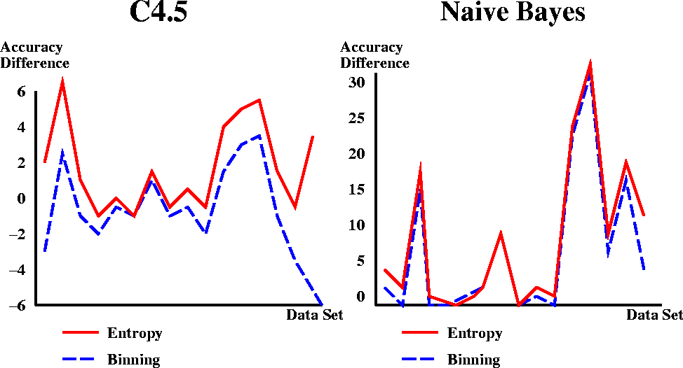
Compare binning, 1R, and entropy-based partitioning
Use C4.5 and Naive Bayes with and without discretizations
Test on 16 UCI datasets, all with at least one continuous feature

The Wrong Way to Experiment

1.: Discretize entire data file
2.: Run 10-fold cross-validation
3.: Report accuracy with and without discretization
4.: Why is this bad?

Results

$\psfig{figure=figures/disc6.ps}$

Large differences in number of intervals. Here is result of diabetes dataset.

Method Accuracy Intervals per attribute

Entropy 76.04 2 4 1 2 3 2 2 3

1R 72.40 6 13 4 6 18 25 41 12

Binning 73.44 8 14 11 11 15 16 18 11

All discretiation methods for Naive Bayes lead to average increase in accuracy
Entropy improves performance on all but three data sets
C4.5, not much change

C4.5-Discretization

Similar to Entropy method
Use C4.5 to build a tree with just the one continuous feature
Apply pruning to find appropriate number of nodes (number of discretization intervals)
Increased pruning confidence beyond default value
Run time is O(lg_1/(1-p m * m lg m), where p is portion of instances split with each decision
Space is O(m)

Sampling

How many training examples do we need?
What type of training examples do we need?
More training examples, better accuracy
PAC learning
Random sampling
Avoid bias

Feature Selection

Selecting a subset of features to give to data mining algorithm.

Motivations

1.: Improve accuracy, many algorithms degrade in performance when given too many features
2.: Improve comprehensibility
3.: Reduce cost and complexity
4.: Investigate with respect to classification task
5.: Scale up to datasets with a large number of features

Example

Credit Approval Database

Initial number of features: 14
Criterion: maximal information gain
Selected features
- Other investments
- Savings account balance
- Bank account
Conclusion: Other 11 attributes not required for predicting class of customer

Feature Selection Criteria

Bayesian approach: no bad features
Information-theoretic approach: prefer features which reduce uncertainty (entropy) in class
Distance measures: maximize distance between prior and posterior distributions of class
Dependence measures: correlation
Consistency measures: find minimum set of features
Accuracy measures: choose set of features which maximizes accuracy

Optimal Features

Given

Inducation algorithm I
Dataset D

The optimal feature subset S^* is set of features that yields in highest-accuracy classifier.

$\begin{displaymath}S^* \;=\; arg max_{S' \subseteq S} acc(I(D_{S'})),\end{displaymath}$

where I(D_S') is the classifier built by I from the dataset D using only features in S'.

The Filter Approach

$\psfig{figure=figures/fs8.ps}$

Select features in a preprocessing step
Generally ignores effects on performance of the learning algorithm

Focus

Almuallim and Dietterich, 1991
Considers all subsets of features
Selects minimal subset sufficient to determine label value of all training instances (MinFeatures bias)
Does not generalize well
Example: use SSN as only feature to discriminate people

Mutual Information

Compute mutual information between each feature and class
MI between two variables
- Average reduction in uncertainty about second variable given value of first variable
- Assume evaluating feature j
- MI weight w_j is
  
  $\begin{displaymath}w_j \;=\; \sum_v \sum_c P(y=c, \;x_j = v) log \frac{P(y=c, x_j=v)}{P(y=c)P(x_j = v)}\end{displaymath}$
- P(y=c) is proportion of training examples in class c
- P(x_j=v) is probability that feature j has value v
More difficult for real-valued features
Each feature is treated independently
Parity function over n features

Relief

Kira and Rendell, 1992
Assign ``relevance'' weight to each feature
Finds all relevant features, not necessarily minimal set
Collect random sample of instances
For each instance
- Find nearest instance of same class (nearest hits)
- Find nearest instance of different class (nearest miss)
- Distance similar to nearest neighbor algorithms
Estimate W[A] of attribute A approximates following value:
W[A] = P(diff value of A $\mid$ nearest instance from different class) -
P(diff value of A $\mid$ nearest instance from same class)
A good attribute should differentiate between instances from different classes and have same value for instances from same class

Pseudocode

set all weights W[A] = 0
for i = 1 to m do
   randomly select instance R
   find nearest hit H and nearest miss M
   for A = 1 to AllAttributes do
      W[A] = W[A] - diff(A,R,H)/m + diff(A,R,M)/m

Here diff(Attribute,Instance1,Instance2) calculates difference between values of the Attribute for two instances.

Discrete attributes: differences is 0 or 1
Continuous atributes: difference is actual difference normalized to [0,1] interval
All weights are in interval [-1,1]

Feature Filtering Using Decision Trees

Generate decision tree using training set
Decision tree usually only uses subset of features
Select features that appear in decision tree
Features useful for decision trees not necessarily useful for nearest neighbor
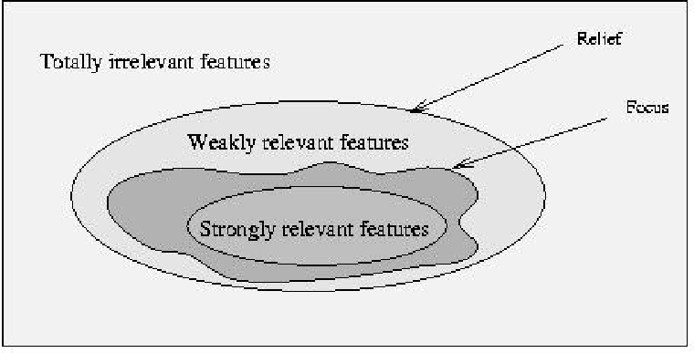
Totally irrelevant features will be removed
Decision trees do not test more than O(lgm) features in a path

Filter Approaches

$\psfig{figure=figures/fs9.ps}$

The Wrapper Approach

$\psfig{figure=figures/fs2.ps}$ 62

Kohavi
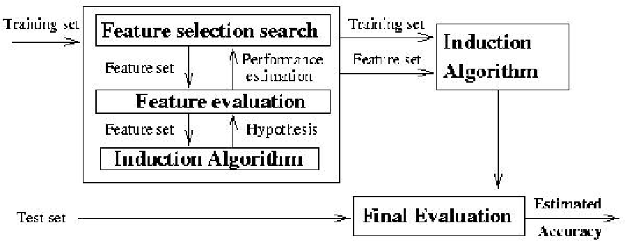
Use induction algorithm as a black box
Conduct search (best-first search here) in the space of subsets
The estimated prediction accuracy using cross-validation is the search heuristic

Experimental Results

Tested wrapper using ID3 and Naive Bayes
Best-first search starting with empty set of features
Final feature subsets evaluated on unseen test instances using five-fold cross validation

Problems

Wrapper very slow
Wrapper has danger of overfitting
Idea for both approaches: weight features, integrate into ML algorithm

Lakshminarayan et al. for feature selection

Used AutoClass class as input feature
No significant performance improvement
AutoClass class was root feature in all of the best trees
AutoClass results used to remove features without significant change in accuracy

In the Spotlight

IBM Advanced Scout

http://www.research.ibm.com/scout

Dealing with Missing Data

Most prediction methods do not handle missing data well
Missing values cannot be multiplied or compared
Solutions
- Use only features with all values
- Use only cases with all values
- These methods lead to bias and insufficient sample sizes
- Fill in missing values during data preparation
  - Replace all values with single global constant
  - Replace each missing value with a single value (single imputation)
  - Replace all missing values with ``unknown category''
    - CART uses this approach
    - Adds additional parameter to estimate
    - Does not reflect fact that missing value is actually part of original value set
    - Can form class just on ``unknown category'' value
  - Problem: The replaced values are frequently not the correct value

Single Imputation

Replace a missing value with its feature mean (mean imputation)
Replace a missing value with its feature and class mean
Replace by expected value calculated from probability distribution
Do not capture uncertainty about true value
Methods can lead to biases

Multiple Imputation

Replace each missing value by vector of M imputed values
Generates M complete data sets
Analyze each set separately

Multiple Imputation Using C4.5

Pretend missing value has all possible values
Weight each value according to frequency among examples in that part of space

Day	Outlook	Temperature	Humidity	Wind	PlayTennis
D1	Sunny	Hot	High	Weak	No
D2	Sunny	Hot	High	Strong	No
D3	Overcast	Hot	High	Weak	Yes
D4	Rain	Mild	High	Weak	Yes
D5	Rain	Cool	Normal	Weak	Yes
D6	Rain	Cool	Normal	Strong	No
D7	Overcast	Cool	Normal	Strong	Yes
D8	Sunny	Mild	High	Weak	No
D9	Sunny	Cool	Normal	Weak	Yes
D10	Rain	Mild	Normal	Weak	Yes
D11	Sunny	Mild	Normal	Strong	Yes
D12	Overcast	Mild	High	Strong	Yes
D13	Overcast	Hot	Normal	Weak	Yes
D14	Rain	Mild	High	?	No

D14 now becomes
D14 Rain Mild High Weak No (weight = 8/13 = 0.62)
D14 Rain Mild High Strong No (weight = 5/13 = 0.38)

Gain(Wind) = I(9/14, 5/14) - Remainder(Wind) Remainder(Wind) =

$\begin{displaymath}\frac{p_{weak} + n_{weak}}{p+n} I(\frac{p_{weak}}{p_{weak} + ... ...ong} + n_{strong}}, \frac{n_{strong}}{p_{strong} + n_{strong}})\end{displaymath}$

= $\frac{8.62}{14}I(\frac{6}{8.62}, \frac{2.62}{8.62}) \;+\; \frac{5.38}{14}I(\frac{3}{5.38}, \frac{2.38}{5.38})$

Lakshminarayan et al.

Working with Honeywell maintenance data
Database contains 4,383 records, each with 82 features
No instance is complete
Only 41 variables have values for more than 50% instances

Methods

AutoClass

Cluster existing data
AutoClass produces probability distribution of features given classes
Replace missing value with value of highest probability for the cluster
AutoClass also ranks variables by influence (useful for feature selection)

CLASS  0 - weight  51   normalized weight 0.249   relative strength  1.64e-10 

 7 33 R SNcn  Log length .........  1.160 ( 5.25e+00  3.41e-02)  2.64e+00 ( 5.16e+00  7.05e-02)
10 36 R SNcn  Log curb-weight ....  1.153 ( 8.08e+00  9.92e-02)  2.57e+00 ( 7.83e+00  1.97e-01)
15  2 D SM    make ...............  0.955  mazda .............. -4.41e+00   1.01e-03  8.27e-02
                             mitsubishi ......... -4.28e+00   8.75e-04  6.33e-02
                             honda .............. -4.28e+00   8.75e-04  6.33e-02
                             subaru ............. -4.20e+00   8.75e-04  5.85e-02
                             volkswagen ......... -4.20e+00   8.78e-04  5.85e-02
                             dodge .............. -3.92e+00   8.75e-04  4.39e-02
                             plymouth ........... -3.67e+00   8.75e-04  3.42e-02
                             isuzu .............. -3.11e+00   8.75e-04  1.96e-02
                             chevrolet .......... -2.83e+00   8.75e-04  1.48e-02
                             alfa-romero ........ -2.83e+00   8.75e-04  1.48e-02
                             renault ............ -2.43e+00   8.75e-04  9.93e-03
                             mercury ............ -1.74e+00   8.90e-04  5.08e-03
                             volvo ..............  1.38e+00   2.13e-01  5.36e-02
                             peugot .............  1.38e+00   2.13e-01  5.36e-02
                             jaguar .............  1.38e+00   5.86e-02  1.48e-02
...

C4.5
- Use learning system to predict value of missing variable
- Feature becomes target, instead of class value
- Variable values cannot be missing for training data

Results

C4.5 yielded 22.6% error rate for target variable
AutoClass yielded 48.7% error rate for target variable
Using top three choices, AutoClass error rate was 18%

Algorithm	Representation	Usage	Adv	Disadv
Association Rule	Prop if-then	discover	simple	slow, rep,
		correlations	no oracle	no predict
Decision Tree	Disj of	prediction	robust prediction,	overfit,
	prop conj		symbolic rules	representation
Neural Network	Nonlinear	prediction	numeric,	overfit, slow,
	numeric f(x)		noisy data	difficult to
				interpret output
Naive Bayes	Est prob	prediction	noisy data,	not effective
			provable answer	in practice
Belief Network	network & CPTs	prediction,	prior info,	slow
		variable influence	prob dist	learn structure
Nearest Neighbor	Instances	prediction	no training,	slow query,
			no fixed bias	redun attributes
			no loss of info	no bias
Clustering	clusters	discover correlations,	no oracle,	difficult to
		discover var influence	find similar features	interpret output
		find sim instances

Method	Accuracy	Intervals per attribute
Entropy	76.04	2	4	1	2	3	2	2	3
1R	72.40	6	13	4	6	18	25	41	12
Binning	73.44	8	14	11	11	15	16	18	11