
rw2pnm can produce
grayscale, one-sided color, or two-sided color output. Here, for the
sake of illustration, we will use an FDTD solution to the problem of a
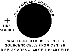
TM line source (i.e., the non-zero components are Ez, Hx, and Hy)
illuminating a circular cylinder which is a perfect electric conductor
(PEC). The line source is driven by a transient pulse and is "close"
to the cylinder. The assumed geometry is

The Finite-Difference Time-Domain (FDTD) program circle.f that generated the raw frames is available. The shell script used to run this simulation and the other details about the generation of the images can be obtained by following this link. (It is not necessary that you understand the FDTD method to understand the animation scheme presented here. However, if you are interested in finding out more about the FDTD method, you can look through the material provided in this database and its accompanying paper -- you may find some useful information there even if you are already an expert in the field.)
In the results presented here only the fields are shown, i.e., the scatterer itself is not "painted." Therefore, since the field is always zero within the scatterer, it may be hard to discern its physical size. If you are interested in making the scatterer, or some other portion of the computational domain, visible, please see the discussion about "sentinel values" in the appendices of the paper.
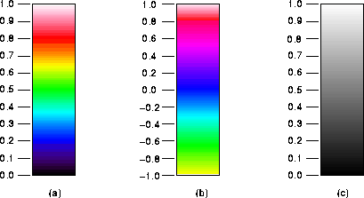
The following figure shows the three color mappings that are used here (keep in mind that it is easy to create your own mappings if you don't like these!). (a) shows the one-sided color map, (b) shows the two-sided color map, and (c) shows the grayscale map.

Note that the two-sided mapping used here differs from the one shown in the paper (which is the one used for the second sample set.) In the following output, two decades of compression were used (see the paper for details regarding the logarithmic compression scheme). Since the color mapping is displayed along the left side of each image and the values are linearly advanced from the lower limit to the upper limit (i.e., between 0 and 1 for grayscale and one-sided output, and between -1 and 1 for two-sided output), the effects of this mapping should be fairly clear---the compression tends to make the output much more sensitive to fluctuations in small values.
 One-sided output:
The absolute value of the normalized field is assumed to be between
zero (black) and one (white). However, as the field varies between
these limits, the displayed values passes through a number of colors.
Click on the "film" below for an MPEG animation that uses a one-sided
color mapping (75 kB):
 Two-sided output:
Here the field is normalized so that it is between negative one and
one. Positive one maps to white, blue is zero, and yellowish green
corresponds to negative one. Note that you can distinguish between
the positive and negative peaks using this mapping while you cannot
distinguish the difference using the other mappings. Click on the
film below for an MPEG animation that uses a two-sided color mapping
(65 kB):
 Grayscale output:
The normalized absolute value of the field is again assumed to be
between zero (black) and one (white). Click on the film below for an
MPEG animation that uses a grayscale mapping (31 kB):
(In addition to the examples presented in the second sample set, additional examples of animations that were created using FDTD modeling can be obtained by following this link. The results present there were created using modified versions of the routines present here. Some obvious differences between the results presented there and those which are produced by the routines presented here are: the computational domain was "split" in the displayed image; a different two-sided mapping was used; and, "sentinel" values were used to show material boundaries. Be forewarned that the files presented there are very large.)

John B.
Schneider, schneidj@eecs.wsu.edu
Patrick J.
Flynn, flynn@ee.eng.ohio-state.edu
Kurt Shlager, kurt.shlager@lmco.com