After the raw output files have been constructed, they must be processed into suitable graphics files. This may be done either concurrently while the data is being generated or in a post-processing step. This stage is depicted in the middle of the flow chart of Fig. 1. Here we will discuss conversion only in the context of post-processing. (A discussion of concurrent processing can be found at the Web site.)
The graphics formats used here are part of the suite of ``portable anymap'' (or PNM) formats that describe raster images. We will be using either grayscale mappings or color mappings. The grayscale output will be designated PGM output (corresponding to ``portable graymap'') while color output will be designated PPM output (corresponding to ``portable pixmap''). Files with these formats can be manipulated in a number of ways using a freely available collection of routines, generally referred to as the pbmplus routines (Appendix C lists sites where these routines can be obtained). Furthermore, these files can easily be converted to a format suitable for printing (such as PostScript) by either using one of the filters supplied in the pbmplus distribution or by using the ghostscript utility found on many systems.
A PNM file starts with a two character ``magic number'' that specifies
the format of the data comprising the image. For example, the magic
number used for color images is P6 indicating byte (binary)
storage of pixel values (the magic number P3 would be used if
pixel values were represented in ASCII). The magic number is followed
by the width, the height, and the maximum gray or color value (all
this ``header'' information is written in ASCII decimal even when the
subsequent data is binary). The width and height are the number of
horizontal and vertical pixels in the image, respectively. The
maximum gray or color value can be used to expand or contract the
dynamic range of an image. However, this is not important for the
task at hand, and hence this value will be fixed at 255. Following
this header information is either the grayscale or RGB (red, green,
blue) information for each pixel in the image. Thus, for a color
image three bytes, representing red, green, and blue, each between 0
and the specified maximum value (255), are given ``width  height'' times. The first three bytes specify the color of the pixel
in the top-left corner of the image and from there proceed left to
right in normal English reading order. If all three bytes are 0, the
pixel will be black; if all are 255, the pixel will be white.
Different colors are obtained by varying the relative values of the R,
G, and B bytes.
height'' times. The first three bytes specify the color of the pixel
in the top-left corner of the image and from there proceed left to
right in normal English reading order. If all three bytes are 0, the
pixel will be black; if all are 255, the pixel will be white.
Different colors are obtained by varying the relative values of the R,
G, and B bytes.
The production of grayscale images is relatively straightforward while the steps involved in creating a color image are slightly more involved. Hence, we will focus the discussion on the generation of color output. As the raw files are translated into PPM files, it is necessary to map field values into RGB values and there are several ways this can be done. It is quite common to quantize the fields so that all values that are between certain limits map to a specified color. Here, instead, we will present an approach where the mapping of fields to color is virtually continuous, i.e., the color changes continuously with continuous changes in field. Unfortunately, it is rather difficult to translate from a field value directly to a desired color using RGB values. In contrast, it is relatively simple to specify desired colors as points in a color space characterized by hue, saturation, and brightness. Assuming for the moment that the brightness is set to unity, we can define a hue-saturation ``color wheel'' as shown in Fig. 2. The center of this wheel corresponds to equal
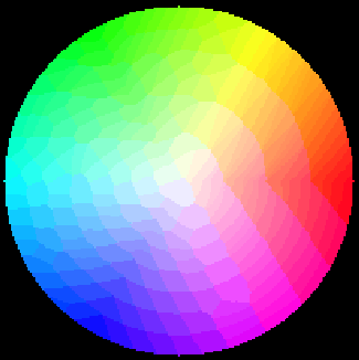
Figure 2: The hue-saturation color wheel (brightness set to unity).
parts of red, green, and blue and is thus white. The distance from
the center is the saturation s, while the angle from the center to a
given point is the hue h. The maximum saturation is unity and the
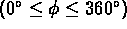
hue is assumed to be between  and
and  . Pure red is
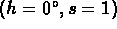 , green corresponds to
 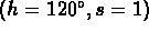 , blue is
 , and white is (h=anything, s=0). Besides hue
and saturation, there is a brightness parameter, usually referred to
as the value or v, that varies between zero and one. If the
brightness is zero, the pixel is black regardless of the hue or
saturation. If the brightness is a small value, the pixel appears
dark. For example, if the saturation is zero (i.e., equal parts of
red, green, and blue) but the brightness is low, the pixel will appear
gray rather than white.
, and white is (h=anything, s=0). Besides hue
and saturation, there is a brightness parameter, usually referred to
as the value or v, that varies between zero and one. If the
brightness is zero, the pixel is black regardless of the hue or
saturation. If the brightness is a small value, the pixel appears
dark. For example, if the saturation is zero (i.e., equal parts of
red, green, and blue) but the brightness is low, the pixel will appear
gray rather than white.
In the conversion of the raw data files to PPM files, a path within
the HSV color space is defined. (The HSV space is defined as a
hexcone, or six-sided pyramid, which can be described naturally in
cylindrical coordinates. However, for the sake of simple
visualization, it may be useful to think of the HSV color space in
terms of a  cylindrical coordinate system where s
corresponds to
cylindrical coordinate system where s
corresponds to 
 , h to
 , and v to z
  . A complete discussion of color spaces is beyond the scope of
this article and the interested reader is directed elsewhere for a
more detailed discussion of the HSV space. For example, see
Computer Graphics: Principles and Practice, (2nd ed.), by J. Foley,
A. van Dam, S. Feiner, and J. Hughes, Addison-Wesley, 1990.) Each
field value is mapped onto this path through the HSV space, thereby
identifying the HSV coordinates of the pixel. Finally, the
coordinates in HSV space are converted to RGB (using a standard
conversion algorithm) and written to the PPM file. Because it is
important in some applications to distinguish between positive and
negative values of the field while in others this distinction is
unimportant, we will define two different color mappings (more can be
constructed if desired). One mapping, shown in
Fig. 3(a), is used for ``one-sided'' output,
. A complete discussion of color spaces is beyond the scope of
this article and the interested reader is directed elsewhere for a
more detailed discussion of the HSV space. For example, see
Computer Graphics: Principles and Practice, (2nd ed.), by J. Foley,
A. van Dam, S. Feiner, and J. Hughes, Addison-Wesley, 1990.) Each
field value is mapped onto this path through the HSV space, thereby
identifying the HSV coordinates of the pixel. Finally, the
coordinates in HSV space are converted to RGB (using a standard
conversion algorithm) and written to the PPM file. Because it is
important in some applications to distinguish between positive and
negative values of the field while in others this distinction is
unimportant, we will define two different color mappings (more can be
constructed if desired). One mapping, shown in
Fig. 3(a), is used for ``one-sided'' output,
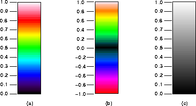
Figure 3: Mapping of fields to pixels. (a) One-sided
color. (b) Two-sided color. (c) Grayscale.
where it is assumed that the normalized absolute value of the field is between zero and unity. The other color mapping, shown in Fig. 3(b), is used for ``two-sided'' output, where it is assumed the normalized field is between -1 and 1. Grayscale mapping, shown in Fig. 3(c), is inherently ``one-sided'' so that that large fields, whether negative or positive, tend to white while small fields tend to black. Please note that once one has a basic understanding of the HSV color space it is simple to construct other color mappings. Therefore, one can easily design color maps that are tailored to a given application. For example, in our modeling of acoustic propagation in water, we chose to make zero pressure correspond to blue. This mapping of blue to ``unperturbed water'' provided a visual context that made the subsequent animations much easier to decipher for those viewing them for the first time then they might have been otherwise.
The main routine that converts the raw files to PGM or PPM files is rw2pnm which is presented in Appendix B. This routine calls the subroutine cmap1 if the one-sided color map is desired, or cmap2 if the two-sided color map is desired. The subroutine hsvrgb is used to convert HSV values to RGB values. (The subroutine listings are also given in Appendix B.) As discussed in more detail below, rw2pnm prompts the user for the base name of the raw files, a normalization value, a scaling parameter, and the desired mapping (i.e., grayscale, one-sided color, or two-sided color). After these are entered, the program uses all of the raw files in sequence to generate the output PNM files. Grayscale files have .pgm appended to the original file name while color output files are postfixed with .ppm. (The rw2pnm program was written in such a way that it can be invoked more than once while working on the same set of files. This permits parallel processing and may be useful when more than one processor can access the disk where the files are stored.)
As the program rw2pnm generates its output, it normalizes each
field value in each frame by the same amount. Typically, the
user-specified normalization would be the  value that was found
during the creation of the raw files (i.e., the largest value written
by the data extraction subroutine). By using this value, the data is
guaranteed to be within the limits assumed by the color mappings. If,
for some reason, a normalized value falls outside of these limits, the
value is mapped to the color corresponding to the appropriate limiting
color and hence it is not imperative that the normalization actually
be greater than the maximum absolute value of the field. In this way,
if the actual
value that was found
during the creation of the raw files (i.e., the largest value written
by the data extraction subroutine). By using this value, the data is
guaranteed to be within the limits assumed by the color mappings. If,
for some reason, a normalized value falls outside of these limits, the
value is mapped to the color corresponding to the appropriate limiting
color and hence it is not imperative that the normalization actually
be greater than the maximum absolute value of the field. In this way,
if the actual  value is not know for a particular set of files,
one need not sift through the entire set seeking the true maximum
value provided that a reasonable guess can be made for a suitable
value.
value is not know for a particular set of files,
one need not sift through the entire set seeking the true maximum
value provided that a reasonable guess can be made for a suitable
value.
In many simulations the fields vary over a large range, and the
mappings shown in Fig. 3 do not provide sufficient
dynamic range. For example, in a small portion of the computational
domain the fields may be large, but over the vast majority of space
the fields may be orders of magnitude smaller. Or, in an animation,
initially the fields may be be large, but as the animation progresses,
the fields may become small (either through absorption or radiation).
These ``small'' values, all close to zero relative to the largest
fields, would appear virtually identical in terms of color. To
provide greater dynamic range, the rw2pnm programs allows the
user to specify a scaling parameter  . If
. If  is zero, ordinary
linear scaling is used. Assuming the user entered the normalization
value
is zero, ordinary
linear scaling is used. Assuming the user entered the normalization
value  , the scaling parameter
  is used to map
logarithmically from the range of field values
is used to map
logarithmically from the range of field values 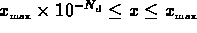 to the range
 . If the field is negative and two-sided output is
required, the sign is preserved, i.e., the range
. If the field is negative and two-sided output is
required, the sign is preserved, i.e., the range 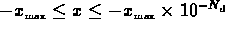 maps to
  . Using this scaling, all fields with an absolute value
less than
. Using this scaling, all fields with an absolute value
less than 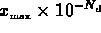 are treated as zero.
This type of scaling can be used to emphasize the variation in small
field values. For example, if the user specifies an
are treated as zero.
This type of scaling can be used to emphasize the variation in small
field values. For example, if the user specifies an  of 4, the
first decade of values, those between
of 4, the
first decade of values, those between  /10 and
  , would be
assigned colors corresponding to those between 0.75 and 1.00 on a
linear scale. The second decade of values, those between
, would be
assigned colors corresponding to those between 0.75 and 1.00 on a
linear scale. The second decade of values, those between  /100
and
/100
and  /10, would be assigned colors corresponding to those between
0.50 and 0.75 on a linear scale, and so on. The same type of scaling
is available if grayscale output is desired. The output from
rw2pnm shows the grayscale or color map used, under the selected
scaling, in a ten-pixel wide column along the left side of each frame.
/10, would be assigned colors corresponding to those between
0.50 and 0.75 on a linear scale, and so on. The same type of scaling
is available if grayscale output is desired. The output from
rw2pnm shows the grayscale or color map used, under the selected
scaling, in a ten-pixel wide column along the left side of each frame.
The following section provides some examples using these mappings and the selectable scaling. In addition, the Animations Web site mentioned in Section 1 provides example MPEG and ``still'' output that was generated using each of the three mappings. The examples are based upon FDTD code that is also available from the Web site.